Ferkans — Interactive Telecom Tutor

LDPC Decoding as Canonical Sum-Product

Low-density parity-check codes are the test case for loopy BP. Their Tanner graphs are bipartite, locally tree-like for large block lengths, and enforced to have girth $\geq 6$ by code design. These are exactly the conditions under which loopy BP shines.

The point of this section is to instantiate the general sum-product rules on the specific factor graph of an LDPC code, derive the log-domain message updates, and understand why the algorithm achieves capacity-approaching performance. We will also introduce density evolution — the asymptotic tool that predicts the decoding threshold without simulation.

Definition:
LDPC Factor Graph

An $(N, K)$ LDPC code has a parity-check matrix $\mathbf{H} \in \mathbb{F}_2^{(N-K) \times N}$ . Its Tanner graph has:

Variable nodes $\{x_1, \ldots, x_N\}$ , one per code bit.
Check nodes $\{c_1, \ldots, c_{N-K}\}$ , one per parity check.
Edge $(x_i, c_m)$ iff $\mathbf{H}_{m,i} = 1$ . The posterior given channel observations $\mathbf{y}$ is $p(\mathbf{x}|\mathbf{y}) \propto \prod_{i=1}^N p(y_i | x_i) \cdot \prod_{m=1}^{N-K} \mathbb{1}\{x_{\partial c_m} \text{ satisfies check } m\}.$

The channel likelihood factors are unary (attached to each variable); the parity-check factors are $d_c$ -ary (degree equals check degree). LDPC-BP alternates updates between variable nodes (combining channel evidence with check messages) and check nodes (enforcing parity).

Theorem: Log-Domain Check-Node Update

Let $L_{j \to c}$ be the incoming LLR on edge $(j, c)$ . The outgoing LLR on edge $(c, i)$ is $L_{c \to i} = 2\, \operatorname{atanh}\!\left(\prod_{j \in \partial c \setminus i} \tanh\!\left(\tfrac{1}{2} L_{j \to c}\right)\right).$ Equivalently, in sign-magnitude form: $L_{c \to i} = \left(\prod_{j \in \partial c \setminus i} \operatorname{sgn}(L_{j \to c})\right) \cdot \phi^{-1}\!\left(\sum_{j \in \partial c \setminus i} \phi(|L_{j \to c}|)\right),$ where $\phi(x) = -\log\tanh(x/2)$ .

The check-node update combines $d_c - 1$ LLRs into one output. The sign of the output is the XOR of the incoming signs (because the check enforces $\sum_j x_j = 0 \bmod 2$ ); the magnitude is dominated by the weakest incoming LLR. The $\phi$ nonlinearity performs a soft-min operation, which is why the min-sum approximation works well.

Proof

Parity-check factor

$f_c(x_{\partial c}) = \mathbb{1}\{\sum_{j \in \partial c} x_j = 0 \bmod 2\}$ . Equivalently, $\prod_{j \in \partial c} (-1)^{x_j} = +1$ — so the XOR of the bits is zero.

Apply sum-product

$\mu_{c \to i}(x_i) \propto \sum_{x_{\partial c \setminus i}: \text{parity ok}} \prod_{j \neq i} \mu_{j \to c}(x_j)$ .

Fourier transform trick

On $\mathbb{F}_2$ , the Fourier transform is $\hat f(k) = \sum_x (-1)^{kx} f(x)$ . Parity constraint $\sum x_j = 0$ becomes $\prod_j \hat\mu_j = \hat\mu_{\text{out}}$ (convolution in real domain = multiplication in Fourier domain).

Express in LLRs

For binary $x$ , $\hat\mu(1) = p(0) - p(1)$ . Writing $p(0) - p(1) = \tanh(L/2)$ where $L = \log(p(0)/p(1))$ : $\tanh(L_{c\to i}/2) = \prod_{j \neq i} \tanh(L_{j \to c}/2)$ . Taking $2\operatorname{atanh}$ gives the stated formula.

,

Theorem: Log-Domain Variable-Node Update

Let $L_i^{\text{ch}} = \log\frac{p(y_i|x_i=0)}{p(y_i|x_i=1)}$ be the channel LLR at bit $i$ . The outgoing LLR on edge $(i, c)$ is $L_{i \to c} = L_i^{\text{ch}} + \sum_{c' \in \partial i \setminus c} L_{c' \to i}.$ The final posterior LLR after $T$ iterations is $L_i^{(T)} = L_i^{\text{ch}} + \sum_{c \in \partial i} L_{c \to i}.$

Variable nodes simply add incoming LLRs — this is the log-domain analog of multiplying probabilities for independent evidence. The extrinsic rule ("exclude the target check") prevents double-counting.

Proof

Apply variable-to-factor message rule

$\mu_{i \to c}(x_i) \propto p(y_i | x_i) \prod_{c' \neq c} \mu_{c' \to i}(x_i)$ . Take log-ratio, using that $L = \log(p(0)/p(1))$ .

Log-ratios add

Since the messages factorize over independent evidence, their log-ratios add: $L_{i \to c} = L_i^{\text{ch}} + \sum_{c' \neq c} L_{c' \to i}$ .

LDPC Sum-Product Decoder (Log-Domain)

Complexity: Per iteration:

O(|\mathcal{E}|)

where

|\mathcal{E}|

is the number of edges in the Tanner graph. For regular

(d_v, d_c)

codes:

|\mathcal{E}| = N d_v

. Memory: one LLR per edge.

Input: channel LLRs L_ch[1..N], parity-check matrix H, max iterations T

Output: decoded codeword x_hat[1..N]

// Initialize messages

for each edge (i, c):

L_{i->c} = L_ch[i]

for t = 1 to T:

// Check-node update

for each check c:

for each i in N(c):

L_{c->i} = 2 * atanh( product over j in N(c){i}:

tanh(L_{j->c} / 2) )

// Variable-node update

for each variable i:

for each c in N(i):

L_{i->c} = L_ch[i] + sum over c' in N(i){c}: L_{c'->i}

// Hard-decision and syndrome check

for each i:

L_total[i] = L_ch[i] + sum over c in N(i): L_{c->i}

x_hat[i] = 0 if L_total[i] >= 0 else 1

if H * x_hat = 0 (mod 2):

return x_hat // Successful decoding

return x_hat // May not be a valid codeword

The min-sum approximation replaces $\phi^{-1}(\sum \phi(|L_j|))$ by $\min_j |L_j|$ , dropping the nonlinearity at a small performance cost (typically 0.3-0.5 dB). Min-sum is the standard in hardware decoders.

LDPC BP Decoding Trajectory: BER vs. Iterations

Run sum-product decoding on a random regular LDPC code over a BSC or AWGN channel. Track the bit-error rate of the current estimate across iterations. Watch the waterfall below the threshold.

Parameters

Block length

N

500

Variable degree

d_v

3

Check degree

d_c

6

Channel SNR (dB)1.5

Max BP iterations30

Definition:
Density Evolution

Density evolution tracks the distribution of BP messages across iterations in the large- $N$ , locally-tree-like limit. Let $P_\ell(L)$ be the density of outgoing variable-to-check LLRs at iteration $\ell$ , and $Q_\ell(L)$ the density of check-to-variable LLRs. For a $(\lambda, \rho)$ irregular ensemble: $Q_\ell = \Gamma(\rho, P_\ell), \qquad P_{\ell+1} = \lambda(P_0 \boxdot Q_\ell),$ where $\Gamma$ and $\boxdot$ are specific functional transforms determined by the check-node and variable-node updates, and $\lambda, \rho$ are the degree distributions.

Density evolution is a scalar (or functional) recursion that predicts the asymptotic BP bit-error rate as a function of channel quality. The threshold $\epsilon^*$ is the largest channel parameter for which $P_\ell \to \delta_\infty$ (perfect recovery in the limit).

Theorem: BP Threshold (BEC)

For the Binary Erasure Channel (BEC) with erasure probability $\epsilon$ and a $(\lambda, \rho)$ irregular LDPC ensemble, the density evolution recursion on the erasure probability $x_\ell$ is $x_{\ell+1} = \epsilon \cdot \lambda\!\big(1 - \rho(1 - x_\ell)\big).$ The BP threshold $\epsilon^*$ is the supremum of $\epsilon$ for which $x_\ell \to 0$ from $x_0 = \epsilon$ .

On the BEC, messages are either "known" or "erased", so the scalar recursion tracks just one number: the probability that a random variable-to-check message is erased. The threshold $\epsilon^*$ is the channel quality at which the recursion first fails to drive erasure to zero — exactly the cliff where decoding breaks down.

Proof

BEC structure

Each message is either fully informative (known bit) or uninformative (erased). A variable-to-check message is erased iff its channel observation is erased and all other check-to-variable messages are erased.

Check-to-variable erasure probability

A check-to-variable message is erased iff any other variable-to-check input to that check is erased: $\Pr(\text{erased}) = 1 - (1 - x_\ell)^{d_c - 1}$ for regular $d_c$ . Irregular version: $1 - \rho(1 - x_\ell)$ .

Variable-to-check update

Erased iff channel erased AND all other checks erased: $\epsilon \cdot \lambda(\text{check erasure})$ .

Threshold as fixed-point boundary

The map $x \mapsto \epsilon \lambda(1 - \rho(1 - x))$ is monotone increasing. $\epsilon^*$ is where $x = 0$ becomes unstable — the cliff. For $\epsilon > \epsilon^*$ , a nonzero fixed point survives: decoding fails asymptotically.

,

Example: Threshold of the (3,6)-Regular LDPC Code on the BEC

Compute the BP threshold of the $(d_v, d_c) = (3, 6)$ regular LDPC ensemble on the BEC. Compare to Shannon's channel-coding bound.

Solution

Specialize density evolution

Regular code: $\lambda(x) = x^{d_v - 1} = x^2$ , $\rho(x) = x^{d_c - 1} = x^5$ . Recursion: $x_{\ell+1} = \epsilon (1 - (1 - x_\ell)^5)^2$ .

Find the threshold

Threshold condition: the map $T(x) = \epsilon(1 - (1-x)^5)^2$ has only fixed point $x = 0$ . For $\epsilon$ just above $\epsilon^*$ , a second fixed point appears. Numerical root-finding yields $\epsilon^* \approx 0.4294$ .

Compare to Shannon

Rate of a $(3, 6)$ -regular code is $R = 1 - d_v/d_c = 0.5$ . Shannon capacity of BEC $(\epsilon)$ is $C = 1 - \epsilon$ ; capacity-achieving requires $\epsilon \leq 1 - R = 0.5$ . The gap $0.5 - 0.4294 = 0.0706$ is the cost of regularity. Irregular codes close this gap further.

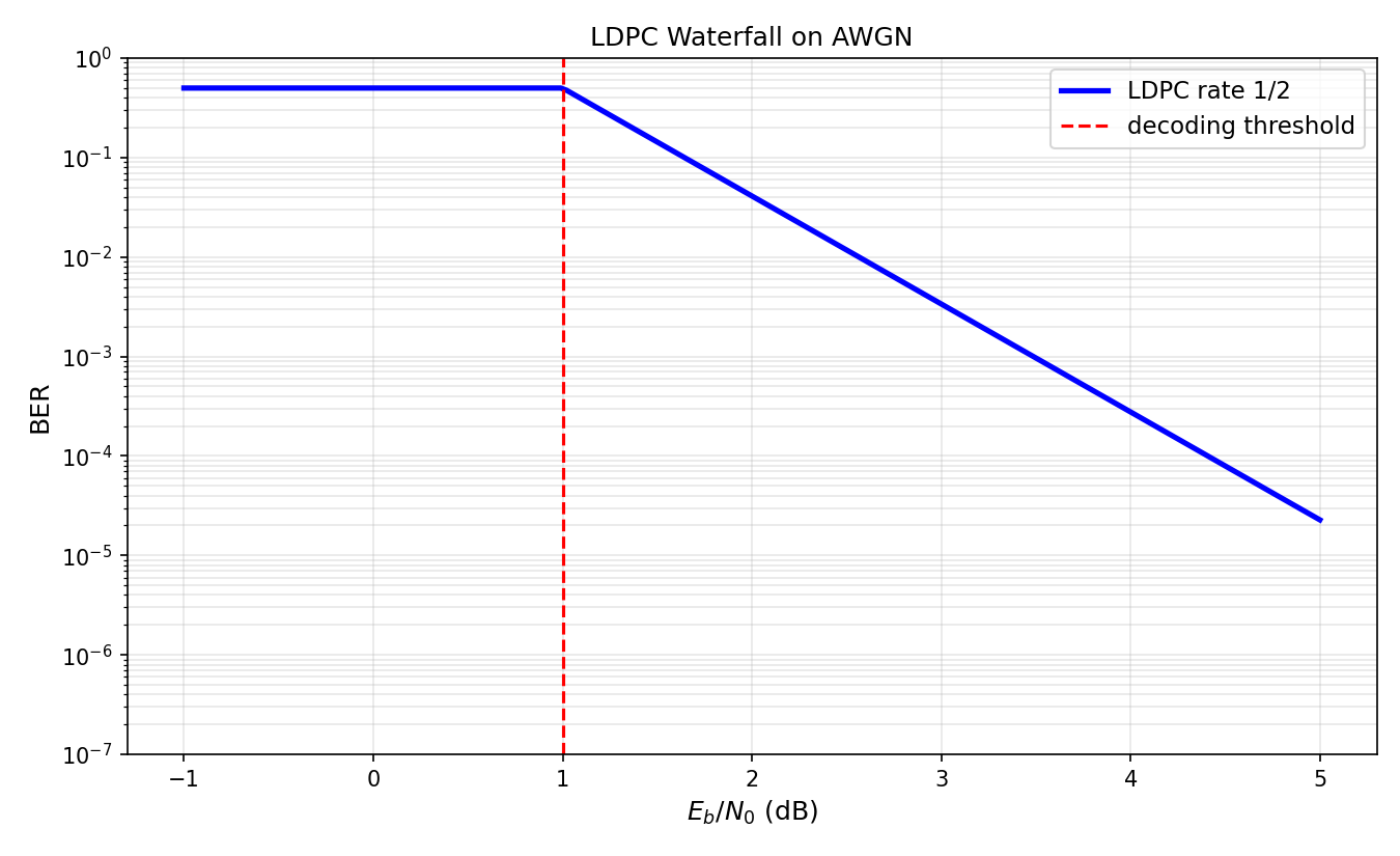
LDPC Waterfall on AWGN — BER vs. SNR for a rate-1/2 LDPC code: the characteristic waterfall curve. Above the threshold (predicted by density evolution), BER drops precipitously; below, it barely moves.

Irregular LDPC Codes Close the Gap

Irregular LDPC codes — with mixed variable-node degrees — can achieve thresholds arbitrarily close to Shannon capacity. The degree distribution is optimized by linear programming on the density evolution recursion (Richardson-Urbanke 2001). Modern 5G LDPC codes use carefully designed irregular ensembles with multi-edge types to optimize both threshold and error floor behavior.

Common Mistake: Uncalibrated Min-Sum Overestimates Confidence

Mistake:

Replacing the exact check-node $\phi$ -operation by plain min-sum without applying a scaling factor.

Correction:

Min-sum systematically overestimates the magnitude of the output LLR. Scale the output by $\alpha \in [0.75, 0.9]$ (determined empirically) to compensate. This is called normalized min-sum and is the standard in hardware decoders. Without scaling, min-sum BP diverges or converges to overconfident errors in the waterfall region.

Historical Note: Gallager, Rediscovery, and 5G

1963-2020

Robert Gallager invented LDPC codes and their iterative decoding in his 1963 PhD thesis — but computational limits of the era made the codes impractical. They were essentially forgotten for 30 years. David MacKay rediscovered them in 1995, showing that Gallager's iterative decoder achieves near-capacity performance at block lengths that modern hardware could handle. Richardson and Urbanke (2001) systematized density evolution, launching the era of code design by threshold optimization. Today LDPC is the channel code in 5G New Radio, in Wi-Fi (802.11n/ac/ax), in DVB-S2, and in NAND flash — a forty-year loop from theory to ubiquitous deployment.

🔧Engineering Note

5G NR LDPC Decoder Specifications

5G NR uses two LDPC base graphs (BG1 and BG2) with lifting factors $Z \in \{2, 3, \ldots, 384\}$ to support block lengths from 40 to 8448 bits and rates from $\approx 1/5$ to $\approx 8/9$ . Commercial decoders use normalized min-sum with $\alpha \approx 0.8$ , layered scheduling, and 15-30 iterations. Throughput exceeds 10 Gb/s in modern 5G modems.

📋 Ref: 3GPP TS 38.212, Section 5.3.2

🎓CommIT Contribution(2004)

EXIT Charts for Iterative Decoder Design

S. ten Brink, G. Kramer, G. Caire — IEEE Trans. Commun.

The CommIT group contributed to developing EXIT (extrinsic information transfer) charts — a graphical dual of density evolution that tracks mutual information rather than message densities. EXIT charts enable joint design of LDPC codes with modulation, equalization, and MIMO detection in iterative receivers. They remain the workhorse tool for designing concatenated iterative systems.

LDPCEXIT chartiterative decodingView Paper →

Quick Check

A check node of degree $d_c$ receives incoming LLRs with magnitudes $\{2, 5, 8, 3\}$ . In normalized min-sum BP with $\alpha = 0.8$ , what is the output magnitude (to a fifth incoming edge)?

$0.8 \cdot 2 = 1.6$

$0.8 \cdot (2+3+5+8) = 14.4$

$0.8 \cdot 8 = 6.4$

$0.8 \cdot (2 \cdot 3 \cdot 5 \cdot 8) = 192$

Correction:

0.8 \cdot 2 = 1.6

Min-sum takes the minimum magnitude (2), times the scaling factor 0.8.

LDPC BP Decoding: Message Flow on a Tanner Graph

Animated BP decoding of an LDPC code. Variable-to-check messages carry accumulated channel evidence; check-to-variable messages enforce parity constraints. Watch the erroneous bits get corrected as iterations proceed.

Key Takeaway

LDPC decoding is canonical loopy BP. The check-node update combines LLRs through a soft-XOR ( $\phi/\phi^{-1}$ or min-sum); the variable-node update adds extrinsic LLRs. Density evolution predicts the exact decoding threshold, and irregular codes push it within hundredths of a dB of Shannon capacity. This is the theoretical backbone of modern channel coding.

Sum-Product for LDPC Decoding

LDPC Decoding as Canonical Sum-Product

Definition: LDPC Factor Graph

Theorem: Log-Domain Check-Node Update

Parity-check factor

Apply sum-product

Fourier transform trick

Express in LLRs

Theorem: Log-Domain Variable-Node Update

Apply variable-to-factor message rule

Log-ratios add

LDPC Sum-Product Decoder (Log-Domain)

LDPC BP Decoding Trajectory: BER vs. Iterations

Parameters

Definition: Density Evolution

Theorem: BP Threshold (BEC)

BEC structure

Check-to-variable erasure probability

Variable-to-check update

Threshold as fixed-point boundary

Example: Threshold of the (3,6)-Regular LDPC Code on the BEC

Specialize density evolution

Find the threshold

Compare to Shannon

LDPC Waterfall on AWGN

Irregular LDPC Codes Close the Gap

Common Mistake: Uncalibrated Min-Sum Overestimates Confidence

Historical Note: Gallager, Rediscovery, and 5G

5G NR LDPC Decoder Specifications

EXIT Charts for Iterative Decoder Design

Quick Check

LDPC BP Decoding: Message Flow on a Tanner Graph

Key Takeaway

Definition:
LDPC Factor Graph

Definition:
Density Evolution