Ferkans — Interactive Telecom Tutor

Why We Need Asymptotic Analysis

In Chapter 13 we derived the LMMSE (Wiener) estimator for linear models $\mathbf{y} = \mathbf{H}\mathbf{x} + \mathbf{w}$ . Its MSE and output SINR can be written explicitly in terms of $\mathbf{H}$ , $\text{SNR}$ , and the input covariance. But in a large MIMO system with, say, $n_t = 64$ transmit and $n_r = 128$ receive antennas, these expressions hide the scaling behavior we actually care about. They depend on the specific realization of $\mathbf{H}$ through eigenvalues that fluctuate from channel to channel.

The point is that as the dimensions grow, the fluctuations vanish. A suitably normalized SINR concentrates around a deterministic value that depends only on the aspect ratio $\beta = n_t/n_r$ and the SNR. This is the power of random matrix theory for wireless systems: we replace the intractable dependence on $\mathbf{H}$ by a scalar fixed-point equation. The result is not a rough estimate — it is sharp, in the sense that the gap between the random SINR and its deterministic limit is $O(1/n_r)$ .

Definition:
Empirical Spectral Distribution

Let $\mathbf{X}_N$ be an $N \times N$ Hermitian matrix with real eigenvalues $\lambda_1, \ldots, \lambda_N$ . Its empirical spectral distribution (ESD) is the random probability measure $F_N(x) = \frac{1}{N} \sum_{k=1}^N \mathbb{1}\{\lambda_k \leq x\}.$ When $F_N(x)$ converges (weakly, almost surely) to a deterministic measure $F(x)$ as $N \to \infty$ , we call $F$ the limiting spectral distribution (LSD).

The ESD summarizes all spectral information into a single measure. Traces of polynomials and inverses of $\mathbf{X}_N$ become integrals against $F_N$ : $\frac{1}{N}\operatorname{tr}(\mathbf{X}_N^{-1}) = \int x^{-1}\,dF_N(x)$ .

Definition:
Stieltjes Transform

The Stieltjes transform of a probability measure $\mu$ on $\mathbb{R}$ is $m_\mu(z) = \int_{\mathbb{R}} \frac{1}{x - z}\,d\mu(x), \qquad z \in \mathbb{C}^+.$ For a Hermitian matrix $\mathbf{X}_N$ with ESD $F_N$ , the associated (random) Stieltjes transform is $m_N(z) = \frac{1}{N}\operatorname{tr}(\mathbf{X}_N - z\mathbf{I})^{-1}$ .

The Stieltjes transform is an analytic function on $\mathbb{C}^+$ (upper half-plane) that encodes the measure $\mu$ . The inversion formula (Plemelj) recovers the density: $f_\mu(x) = \frac{1}{\pi}\lim_{\eta \to 0^+} \operatorname{Im}\, m_\mu(x + j\eta)$ . Convergence of the ESD is equivalent to pointwise convergence of $m_N(z)$ on $\mathbb{C}^+$ .

Theorem: Marchenko-Pastur Law

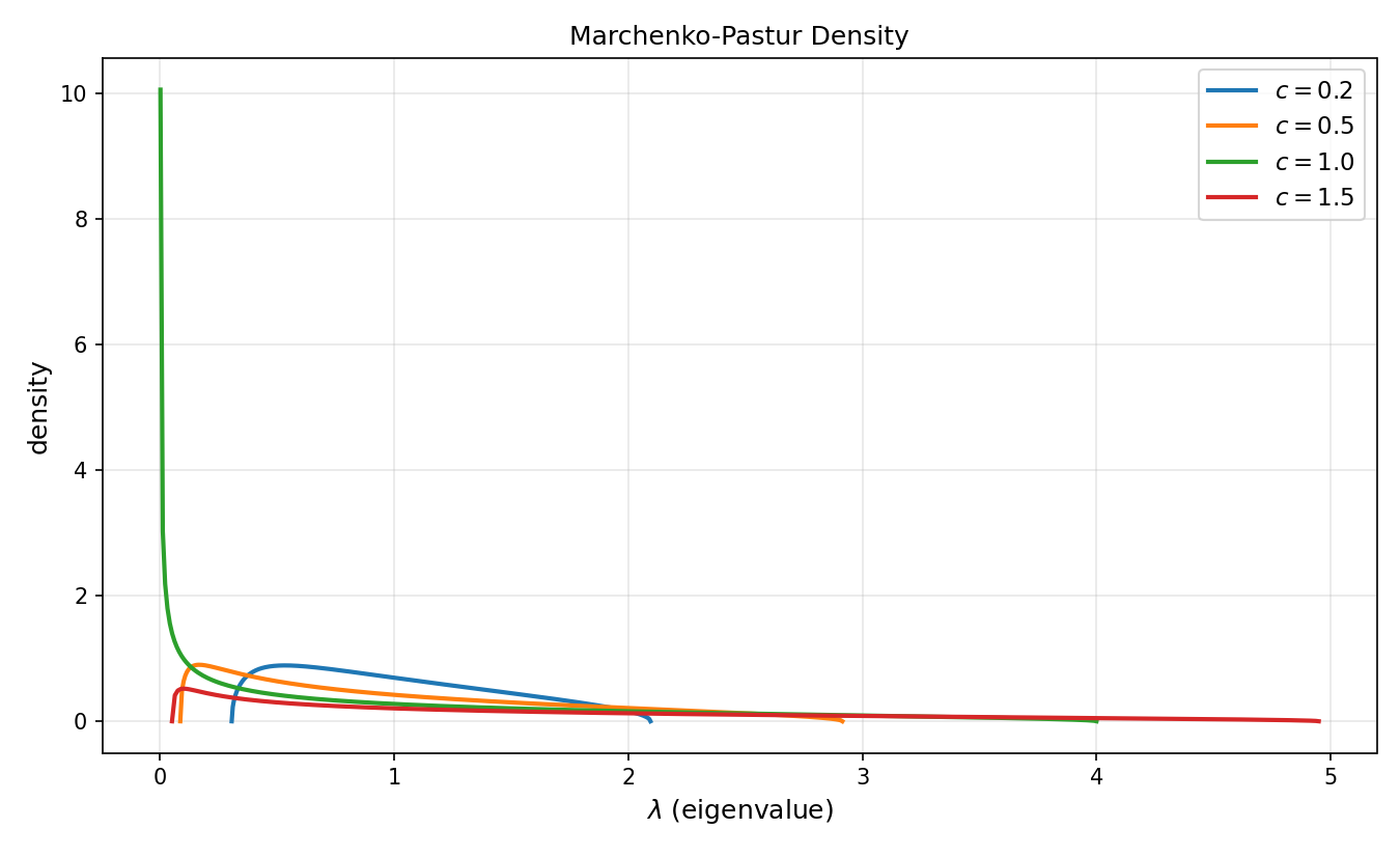
Let $\mathbf{H}$ be an $N \times M$ matrix whose entries are i.i.d. complex (or real) with mean zero, variance $1/N$ , and finite fourth moment. Let $\beta = M/N$ and consider the Gram matrix $\mathbf{W} = \mathbf{H}\mathbf{H}^H$ . As $N, M \to \infty$ with $M/N \to \beta \in (0, \infty)$ , the ESD of $\mathbf{W}$ converges almost surely to the Marchenko-Pastur distribution with density $f_{\text{MP}}(x) = \left(1 - \frac{1}{\beta}\right)^+ \delta(x) + \frac{\sqrt{(x - \lambda_-)^+ (\lambda_+ - x)^+}}{2\pi x}, \quad \lambda_\pm = (1 \pm \sqrt{\beta})^2.$

The eigenvalues of a large i.i.d. Gram matrix do not cluster around the mean $\mathbb{E}[\lambda] = \beta$ . They spread out over the interval $[\lambda_-, \lambda_+]$ , and the width of this interval is $4\sqrt{\beta}$ . When $\beta < 1$ , the matrix is tall and full rank; when $\beta > 1$ , there are $(1 - 1/\beta) N$ zero eigenvalues because $\mathbf{H}\mathbf{H}^H$ is rank-deficient. The point is that a large random MIMO channel has an extreme spectrum — its smallest singular value approaches $|1 - \sqrt{\beta}|$ , not zero, provided $\beta \neq 1$ .

Proof

Set up the fixed-point equation for the Stieltjes transform

Let $m_N(z) = \frac{1}{N}\operatorname{tr}(\mathbf{H}\mathbf{H}^H - z\mathbf{I})^{-1}$ . Using the Sherman-Morrison formula, peel off one column $\mathbf{h}_k$ of $\mathbf{H}$ and write $\left[\mathbf{H}\mathbf{H}^H - z\mathbf{I}\right]^{-1}_{kk} = \frac{1}{\mathbf{h}_k^H \mathbf{h}_k - z - \mathbf{h}_k^H \mathbf{A}_k^{-1} \mathbf{h}_k},$ where $\mathbf{A}_k$ is the matrix with column $k$ removed.

Concentrate the quadratic forms

For $\mathbf{h}_k$ i.i.d. with variance $1/N$ , the quadratic form $\mathbf{h}_k^H \mathbf{A}_k^{-1} \mathbf{h}_k$ concentrates around $\frac{1}{N}\operatorname{tr}(\mathbf{A}_k^{-1})$ which in turn converges to $m(z)$ (by the rank-one perturbation lemma, removing one column does not change the Stieltjes transform in the limit).

Derive the Marchenko-Pastur equation

Summing the diagonal entries and taking $N \to \infty$ : $m(z) = \frac{\beta}{-z(1 + m(z)) + (\beta - 1) - z\beta m(z)} \quad \text{(rearranging)}.$ This simplifies to the quadratic $\beta z\, m(z)^2 + (z - (\beta - 1))\, m(z) + 1 = 0.$

Invert to obtain the density

Solving the quadratic and taking the root with $\operatorname{Im}(m) > 0$ on $\mathbb{C}^+$ , then applying Plemelj's inversion formula $f(x) = \frac{1}{\pi}\operatorname{Im}\, m(x + j0^+)$ , yields the density in the theorem.

,

Marchenko-Pastur Density for Several Aspect Ratios — Density $f_{\text{MP}}(x)$ for $\beta \in \{0.25, 0.5, 1.0, 2.0\}$ . At $\beta = 1$ the density diverges at $x = 0$ ; this is the hard edge that makes square Gaussian matrices poorly conditioned.

Marchenko-Pastur: Empirical vs. Asymptotic Spectrum

Compare the eigenvalue histogram of a finite random Gram matrix $\mathbf{W} = \mathbf{H}\mathbf{H}^H$ (with $\mathbf{H}$ i.i.d. $\mathcal{CN}$ ) to the Marchenko-Pastur density. Adjust the dimensions and watch the histogram lock onto the limit.

Parameters

Number of rows

N

200

Aspect ratio

\beta = M/N

0.5

Number of independent trials (averaged)1

Definition:
LMMSE Detector SINR (Finite $n_r$ )

Consider the MIMO channel $\mathbf{y} = \mathbf{H}\mathbf{x} + \mathbf{w}$ with $\mathbf{x} \sim \mathcal{CN}(\mathbf{0}, \mathbf{I})$ and $\mathbf{w} \sim \mathcal{CN}(\mathbf{0}, \sigma^2\mathbf{I})$ . The LMMSE detector for stream $k$ is $\hat{x}_k = \mathbf{g}_k^H \mathbf{y}$ with $\mathbf{G} = \mathbf{H}^{H}(\mathbf{H}\mathbf{H}^{H} + \sigma^2\mathbf{I})^{-1}$ . Equivalently, $\mathbf{G} = (\mathbf{H}^{H}\mathbf{H} + \sigma^2\mathbf{I})^{-1}\mathbf{H}^{H}$ . Its output SINR for stream $k$ is $\operatorname{SINR}_k = \mathbf{h}_k^H (\mathbf{H}_{(k)}\mathbf{H}_{(k)}^{H} + \sigma^2\mathbf{I})^{-1} \mathbf{h}_k,$ where $\mathbf{H}_{(k)}$ is $\mathbf{H}$ with column $k$ removed.

Theorem: Deterministic Equivalent of the LMMSE SINR

Assume the entries of $\mathbf{H}$ are i.i.d. $\mathcal{CN}(0, 1/n_r)$ . In the large-system limit $n_t, n_r \to \infty$ with $n_t/n_r \to \beta$ , the output SINR of the LMMSE detector on any stream converges almost surely to $\operatorname{SINR}^\infty(\beta, \text{SNR}) = \frac{1}{\text{SNR}^{-1} \cdot m(-\text{SNR}^{-1}) + \text{correction}} - 1,$ where $m(z)$ satisfies the fixed-point equation $m(z) = \left(-z + \frac{\beta}{1 + m(z)}\right)^{-1}.$ Equivalently, the limiting SINR is the unique positive solution of $\gamma = \frac{\text{SNR}}{1 + \beta \cdot \frac{\gamma}{1 + \gamma}}.$

The deterministic equivalent replaces a random quantity (the SINR, which depends on the channel realization) by a scalar depending only on $\beta$ and $\text{SNR}$ . The fixed-point $\gamma = \text{SNR}/(1 + \beta\gamma/(1+\gamma))$ admits an elegant interpretation: in the large-system limit each stream "sees" an effective interference-plus-noise with variance equal to a self-consistent function of its own SINR. The circular definition resolves into a quadratic. This is the simplest instance of the replica symmetric prediction in random matrix theory.

Proof

Rewrite the SINR using the matrix inversion lemma

By the Sherman-Morrison formula, $\operatorname{SINR}_k = \mathbf{h}_k^H(\mathbf{H}\mathbf{H}^H + \sigma^2\mathbf{I} - \mathbf{h}_k\mathbf{h}_k^H)^{-1}\mathbf{h}_k$ equals $\mathbf{h}_k^H \mathbf{M}^{-1} \mathbf{h}_k / (1 - \mathbf{h}_k^H \mathbf{M}^{-1}\mathbf{h}_k)$ appropriately. After algebra, $\operatorname{SINR}_k = \mathbf{h}_k^H(\mathbf{H}\mathbf{H}^H + \sigma^2\mathbf{I})^{-1}\mathbf{h}_k / (1 - \text{that}$ ).

Trace lemma

For $\mathbf{h}_k$ independent of $\mathbf{M}$ with i.i.d. entries of variance $1/n_r$ , the quadratic form concentrates: $\mathbf{h}_k^H \mathbf{M}^{-1} \mathbf{h}_k - \frac{1}{n_r}\operatorname{tr}(\mathbf{M}^{-1}) \xrightarrow{a.s.} 0$ . The normalized trace converges to the Stieltjes transform: $\frac{1}{n_r}\operatorname{tr}(\mathbf{H}\mathbf{H}^H + \sigma^2\mathbf{I})^{-1} \to m(-\sigma^2)$ .

Close the fixed-point equation

Writing $\text{SNR} = 1/\sigma^2$ and the Marchenko-Pastur fixed-point equation for $m(-1/\text{SNR})$ , eliminating $m$ , and using $\operatorname{SINR}^\infty = \text{SNR} - m \cdot \text{SNR}^{2}$ (after algebra) yields the cubic-free form $\gamma = \text{SNR}/(1 + \beta\gamma/(1+\gamma))$ .

Verify the fixed-point is unique

The map $T(\gamma) = \text{SNR}/(1 + \beta\gamma/(1+\gamma))$ is strictly decreasing in $\gamma$ for $\gamma > 0$ , so it has a unique fixed point. Standard RMT arguments (Tse-Hanly 1999) show that $\operatorname{SINR}_k \xrightarrow{a.s.} \gamma^*$ .

, ,

Example: Solving the LMMSE Fixed-Point Equation

For a MIMO system with $\beta = 0.5$ (two receive antennas per transmit stream) and $\text{SNR} = 10$ dB, compute the asymptotic LMMSE SINR $\gamma^*$ . Compare to the single-user SISO rate $\log_2(1+\text{SNR})$ .

Solution

Set up the fixed point

$\text{SNR} = 10$ dB $= 10$ . The fixed-point equation is $\gamma = \frac{10}{1 + 0.5 \cdot \gamma/(1+\gamma)}$ .

Solve the quadratic

Multiply out: $\gamma (1 + \frac{0.5\gamma}{1+\gamma}) = 10$ , so $\gamma(1+\gamma) + 0.5 \gamma^2 = 10(1+\gamma)$ . Expanding: $1.5\gamma^2 + \gamma - 10 - 10\gamma = 0$ , i.e., $1.5\gamma^2 - 9\gamma - 10 = 0$ . The positive root is $\gamma^* = (9 + \sqrt{81 + 60})/3 = (9 + \sqrt{141})/3 \approx 6.96$ .

Convert to spectral efficiency

The per-stream rate is $\log_2(1 + \gamma^*) \approx \log_2(7.96) \approx 2.99$ bits/s/Hz. The single-user SISO rate at the same SNR is $\log_2(11) \approx 3.46$ bits/s/Hz. The loss is about 0.47 bits per stream — this is the price paid for multi-stream interference even with optimal linear processing.

Total spectral efficiency

With $n_t$ streams the total rate scales as $n_t \cdot 2.99$ , so doubling $n_r$ (reducing $\beta$ from 1 to 0.5) is worth much more than a single SISO link even though the per-stream rate drops.

Why the Fixed-Point is Benign

The fixed-point equation $\gamma = \text{SNR}/(1 + \beta\gamma/(1+\gamma))$ is not a convex optimization per se, but the map whose fixed point we seek is a contraction on $(0, \infty)$ in the metric $d(\gamma_1, \gamma_2) = |\log(\gamma_1/\gamma_2)|$ . Fixed-point iteration converges globally and monotonically from any starting point — a reliable property that matters when we need to evaluate the limit over thousands of $(\beta, \text{SNR})$ pairs for system design.

Deterministic Equivalent vs. Monte Carlo

Compare the asymptotic SINR predicted by the fixed-point equation to the empirical SINR distribution over random $\mathbf{H}$ realizations. As $n_r$ grows, the empirical distribution concentrates at the fixed point.

Parameters

Aspect ratio

\beta = n_t/n_r

0.5

SNR (dB)10

Receive antennas

n_r

32

⚠️Engineering Note

Large-System Approximations in System Design

System designers routinely use large-system deterministic equivalents for early-stage link budget analysis. For $n_r \geq 16$ , the prediction error of the asymptotic SINR formula is typically under 0.3 dB. This allows sweeping thousands of configurations analytically rather than running Monte Carlo.

Practical Constraints

•
Formulas assume i.i.d. Rayleigh fading — correlated channels require the generalized Silverstein equation.
•
Per-realization outage behavior is lost — only ergodic metrics are captured.
•
Deterministic equivalents are asymptotic: below $n_r \approx 8$ the variance of the SINR matters.

Historical Note: From Nuclear Physics to Wireless

1967-1999

The Marchenko-Pastur law (1967) was published in a Soviet mathematics journal with no applied motivation — it generalized Wigner's semicircle law from nuclear physics to rectangular matrices. Three decades later, David Tse and Steve Hanly (1999) recognized that the same distribution governs the SINR of CDMA receivers when the number of users and the spreading gain both grow to infinity. Sergio Verdú and Shlomo Shamai independently obtained closely related results. This opened a highly productive line of research that is now the standard analytical tool for massive MIMO and cell-free networks.

Why This Matters: Cell-Free Massive MIMO

In cell-free massive MIMO, each user is served by a large pool of distributed access points. The combined channel matrix is thin and tall, with $\beta \ll 1$ . The Marchenko-Pastur analysis here predicts the achievable per-user SINR after centralized LMMSE processing, and informs the centralized-vs-distributed tradeoff explored in Book MIMO Chapter 18.

Common Mistake: Forgetting the Aspect Ratio Regime

Mistake:

Applying the Marchenko-Pastur formulas in the square regime $\beta \approx 1$ , where the density diverges at $x = 0$ and small eigenvalues dominate the MSE.

Correction:

At $\beta = 1$ , the smallest eigenvalue of $\mathbf{H}\mathbf{H}^{H}$ scales as $1/n_r$ , so the LMMSE matrix inversion is ill-conditioned. The deterministic equivalent is still valid, but the constants in the $O(1/n_r)$ error bound blow up as $\beta \to 1$ . In practice, stay away from $\beta = 1$ — add regularization or use more receive antennas.

Quick Check

For $\beta = 0.25$ (four times more rows than columns), what is the lower edge $\lambda_-$ of the Marchenko-Pastur density?

$\lambda_- = 0.25$

$\lambda_- = 0$

$\lambda_- = 0.5$

$\lambda_- = 1 - 2\sqrt{\beta}$

Correction:

\lambda_- = 0.25

$\lambda_- = (1 - \sqrt{\beta})^2 = (1 - 0.5)^2 = 0.25$ .

The Marchenko-Pastur Law Emerging

Animated convergence of the eigenvalue histogram of

\mathbf{H}\mathbf{H}^{H}

to the Marchenko-Pastur density as

N

grows. The random spectrum locks onto the deterministic limit before your eyes.

Key Takeaway

In the large-system limit, the random output SINR of an LMMSE detector on an i.i.d. Rayleigh MIMO channel concentrates around a deterministic value characterized by a simple scalar fixed-point equation in $\beta$ and $\text{SNR}$ . This replaces per-realization simulation with an analytic formula — an indispensable tool for massive MIMO system design.

🎓CommIT Contribution(2011)

Deterministic Equivalents for Correlated Channels

R. Couillet, M. Debbah, G. Caire — IEEE Trans. Inform. Theory

The CommIT group contributed to extending deterministic-equivalent techniques from the classical i.i.d. Marchenko-Pastur setting to isometric (Haar) precoders and correlated channels. This is the mathematical foundation behind many of the system-level predictions in Book MIMO.

random matrixdeterministic equivalentlarge systemView Paper →

Large-System Analysis of MIMO Detection

Why We Need Asymptotic Analysis

Definition: Empirical Spectral Distribution

Definition: Stieltjes Transform

Theorem: Marchenko-Pastur Law

Set up the fixed-point equation for the Stieltjes transform

Concentrate the quadratic forms

Derive the Marchenko-Pastur equation

Invert to obtain the density

Marchenko-Pastur Density for Several Aspect Ratios

Marchenko-Pastur: Empirical vs. Asymptotic Spectrum

Parameters

Definition: LMMSE Detector SINR (Finite nrn_rnr​)

Theorem: Deterministic Equivalent of the LMMSE SINR

Rewrite the SINR using the matrix inversion lemma

Trace lemma

Close the fixed-point equation

Verify the fixed-point is unique

Example: Solving the LMMSE Fixed-Point Equation

Set up the fixed point

Solve the quadratic

Convert to spectral efficiency

Total spectral efficiency

Why the Fixed-Point is Benign

Deterministic Equivalent vs. Monte Carlo

Parameters

Large-System Approximations in System Design

Historical Note: From Nuclear Physics to Wireless

Why This Matters: Cell-Free Massive MIMO

Common Mistake: Forgetting the Aspect Ratio Regime

Quick Check

The Marchenko-Pastur Law Emerging

Key Takeaway

Deterministic Equivalents for Correlated Channels

Definition:
Empirical Spectral Distribution

Definition:
Stieltjes Transform

Definition:
LMMSE Detector SINR (Finite $n_r$ )