Ferkans — Interactive Telecom Tutor

Sharp Thresholds in Sparse Recovery

In Chapter 14 we proved that the LASSO recovers a sparse signal $\mathbf{x}^\star$ from $\mathbf{y} = \mathbf{A}\mathbf{x}^\star + \mathbf{w}$ provided the sensing matrix satisfies the restricted isometry property (RIP) and the number of measurements exceeds $M \gtrsim s \log(N/s)$ .

That bound is sufficient, and it captures the correct scaling. But for a system designer, the multiplicative constants are what matter: does one need $M = 4s\log(N/s)$ or $M = 20s\log(N/s)$ ? The point of this section is that for Gaussian $\mathbf{A}$ , the gap between success and failure is not gradual — it is a phase transition with a sharp threshold that can be computed exactly. The Donoho-Tanner curve tells the designer whether their $(M, N, s)$ triple lies on the good side or the bad side of the cliff.

Definition:
Phase Transition Regime

Consider the noiseless sparse recovery problem $\hat{\mathbf{x}} = \arg\min \|\mathbf{x}\|_1 \quad \text{s.t.} \quad \mathbf{A}\mathbf{x} = \mathbf{y},$ where $\mathbf{A} \in \mathbb{R}^{M \times N}$ has i.i.d. $\mathcal{N}(0, 1/M)$ entries and $\mathbf{x}^\star$ is $s$ -sparse. Define the undersampling ratio $\delta = M/N \in (0, 1]$ and the sparsity ratio $\rho = s/M$ . The phase transition regime is the double asymptotic $N \to \infty$ with $(\delta, \rho)$ fixed.

$\delta$ measures how aggressively we undersample relative to the ambient dimension. $\rho$ measures how many of the measurements are "spent" per nonzero entry. The regime $\delta \to 0$ with $\rho$ bounded is the high-compression limit.

Theorem: Donoho-Tanner Phase Transition

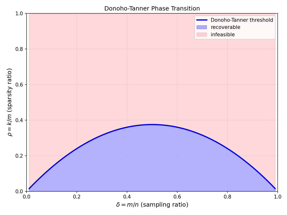
For $\mathbf{A}$ with i.i.d. Gaussian entries, there exists a deterministic curve $\rho^*(\delta): (0, 1] \to (0, 1]$ such that in the double limit $N \to \infty$ : $\Pr(\hat{\mathbf{x}} = \mathbf{x}^\star) \to \begin{cases} 1 & \rho < \rho^*(\delta) \\ 0 & \rho > \rho^*(\delta) \end{cases}$ The curve $\rho^*(\delta)$ is characterized implicitly by the solution of a geometric covering problem involving random convex polytopes (Donoho, 2005). Specifically, $\rho^*(\delta)$ is the fraction of $(M-1)$ -faces of the cross-polytope $\mathbb{B}_1^N$ that survive random projection to $\mathbb{R}^M$ .

The transition is sharp: for any $\epsilon > 0$ , the probability of recovery jumps from below $\epsilon$ to above $1 - \epsilon$ as $\rho$ crosses $\rho^*(\delta)$ in a band of width $O(1/\sqrt{N})$ . Below the curve, $\ell_1$ minimization recovers $\mathbf{x}^\star$ exactly with probability one in the limit; above it, recovery fails. The curve captures the best possible tradeoff between measurements and sparsity for any convex-relaxation recovery method over Gaussian matrices.

Proof

Geometric formulation (combinatorial geometry)

$\ell_1$ -minimization succeeds at $\mathbf{x}^\star$ iff $\mathbf{x}^\star$ lies on a face of $\mathbb{B}_1^N$ (the $\ell_1$ ball) whose image under $\mathbf{A}$ is also a face of $\mathbf{A}(\mathbb{B}_1^N)$ . The number of such "surviving" faces is a classical random-polytope quantity.

Affinely invariant face-counting

By the Affentranger-Schneider face-counting formulas for random polytopes, the expected fraction of $k$ -faces surviving is expressible in terms of external angles. These angles are computed via a scalar integral.

Sharpness via concentration

The number of violated conditions concentrates around its mean with variance $O(N)$ , so fluctuations vanish on the $N \to \infty$ scale. The sharp threshold follows.

Weak and strong thresholds

The theorem above concerns the weak threshold (recovery for a specific generic $\mathbf{x}^\star$ ). A strong threshold $\rho_S^*(\delta)$ guarantees uniform recovery for all $s$ -sparse vectors simultaneously and lies strictly below $\rho^*(\delta)$ .

, ,

The Donoho-Tanner Phase Transition Curve — Phase transition curve $\rho^*(\delta)$ for the noiseless sparse recovery problem with Gaussian $\mathbf{A}$ . Below the curve, $\ell_1$ minimization succeeds almost surely; above, it fails almost surely. The band around the curve is $O(N^{-1/2})$ wide.

Donoho-Tanner Curve and Empirical Phase Diagram

Overlay the theoretical curve $\rho^*(\delta)$ with simulated success probability for finite $N$ . Move the slider to see the transition sharpen as $N$ grows.

Parameters

Signal dimension

N

200

Monte Carlo trials per

(\delta, \rho)

15

Grid resolution15

Example: Sizing a Sparse Recovery System

You need to reconstruct a signal with $N = 10{,}000$ coefficients of which $s = 200$ are nonzero. How many Gaussian measurements $M$ does the Donoho-Tanner theory predict you need, assuming a weak-threshold operating point?

Solution

Estimate the required $\rho$

Pick a target $\delta$ and solve $\rho^*(\delta) = s/M = 200/M$ . For $\delta = 0.1$ (i.e., $M = 1000$ ), the Donoho-Tanner table gives $\rho^*(0.1) \approx 0.193$ . Thus $s/M \leq 0.193$ requires $M \geq 1036$ .

Try $\delta = 0.2$

At $\delta = 0.2$ ( $M = 2000$ ), $\rho^*(0.2) \approx 0.277$ . So $s/M = 0.1 \ll 0.277$ : comfortably below. But we used twice as many measurements. The operating region depends on how close to the cliff you want to be.

Interpretation

$M = 1040$ is the minimum in the noiseless, Gaussian, asymptotic sense. In practice one adds a safety margin (30-50%) for finite- $N$ effects and noise, yielding $M \approx 1500$ . For a designer this translates directly into the number of sensors, ADC channels, or RF chains required.

Sparse Recovery: Theoretical vs. Practical Thresholds

Method	Weak threshold $\rho^*(\delta)$	Noise robust?	Complexity
$\ell_1$ / LASSO	Donoho-Tanner curve (tight)	Yes (LASSO)	$O(N^3)$
Orthogonal Matching Pursuit	Slightly below DT curve	Moderate	$O(s \cdot MN)$
Approximate Message Passing (AMP)	Matches DT curve asymptotically	Yes (state evolution)	$O(MN)$ per iter
CoSaMP / IHT	Below DT curve	Yes	$O(MN)$ per iter

AMP Saturates the Curve

Approximate Message Passing (Chapter 20) achieves the Donoho-Tanner curve with $O(MN)$ per-iteration complexity — dramatically faster than interior-point solvers for LASSO. This is possible because AMP's state evolution recursion provably tracks the LASSO solution in the high-dimensional limit. The practical implication: Donoho-Tanner is not just a theoretical benchmark; it is operationally achievable on problems with $N = 10^5$ or larger.

Common Mistake: Non-Gaussian Sensing Matrices

Mistake:

Applying the Donoho-Tanner curve to structured sensing matrices (partial Fourier, Bernoulli, binary) without adjustment.

Correction:

The curve was derived for i.i.d. Gaussian $\mathbf{A}$ . Partial Fourier matrices (used in MRI) exhibit a different, slightly more conservative phase transition. Bernoulli $\pm 1/\sqrt{M}$ matrices are very close to Gaussian but not identical. Sub-Gaussian concentration ensures the curve is a good approximation, but constants should be verified by simulation before committing to a design.

Phase transition (in sparse recovery)

A sharp threshold in the $(\delta, \rho) = (M/N, s/M)$ plane separating regimes of successful and failed recovery. The width of the transition band shrinks as $O(1/\sqrt{N})$ , so in the high-dimensional limit it is a cliff.

Quick Check

A sensing system uses $M = 500$ random Gaussian measurements on an $N = 5000$ dimensional signal. The Donoho-Tanner curve gives $\rho^*(0.1) \approx 0.19$ . What is the maximum $s$ -sparse signal the system can reliably recover?

$s \leq 95$

$s \leq 500$

$s \leq 950$

$s \leq 19$

Correction:

s \leq 95

$\rho = s/M \leq 0.19$ gives $s \leq 0.19 \times 500 = 95$ .

🔧Engineering Note

Safety Margins in Practice

In deployed systems, operate with $\rho$ at roughly 60-70% of $\rho^*(\delta)$ to tolerate noise, model mismatch, and finite- $N$ effects. AMP-based recovery with online noise-variance estimation is the standard choice when $N > 10^4$ .

📋 Ref: Donoho-Maleki-Montanari 2009

Key Takeaway

The Donoho-Tanner phase transition is a sharp cliff in the $(\delta, \rho)$ plane: below the curve, $\ell_1$ -recovery succeeds with probability one; above, it fails with probability one. For Gaussian sensing matrices the curve is known explicitly. It is the gold standard benchmark for any practical sparse-recovery algorithm.

Phase Transitions in Sparse Recovery